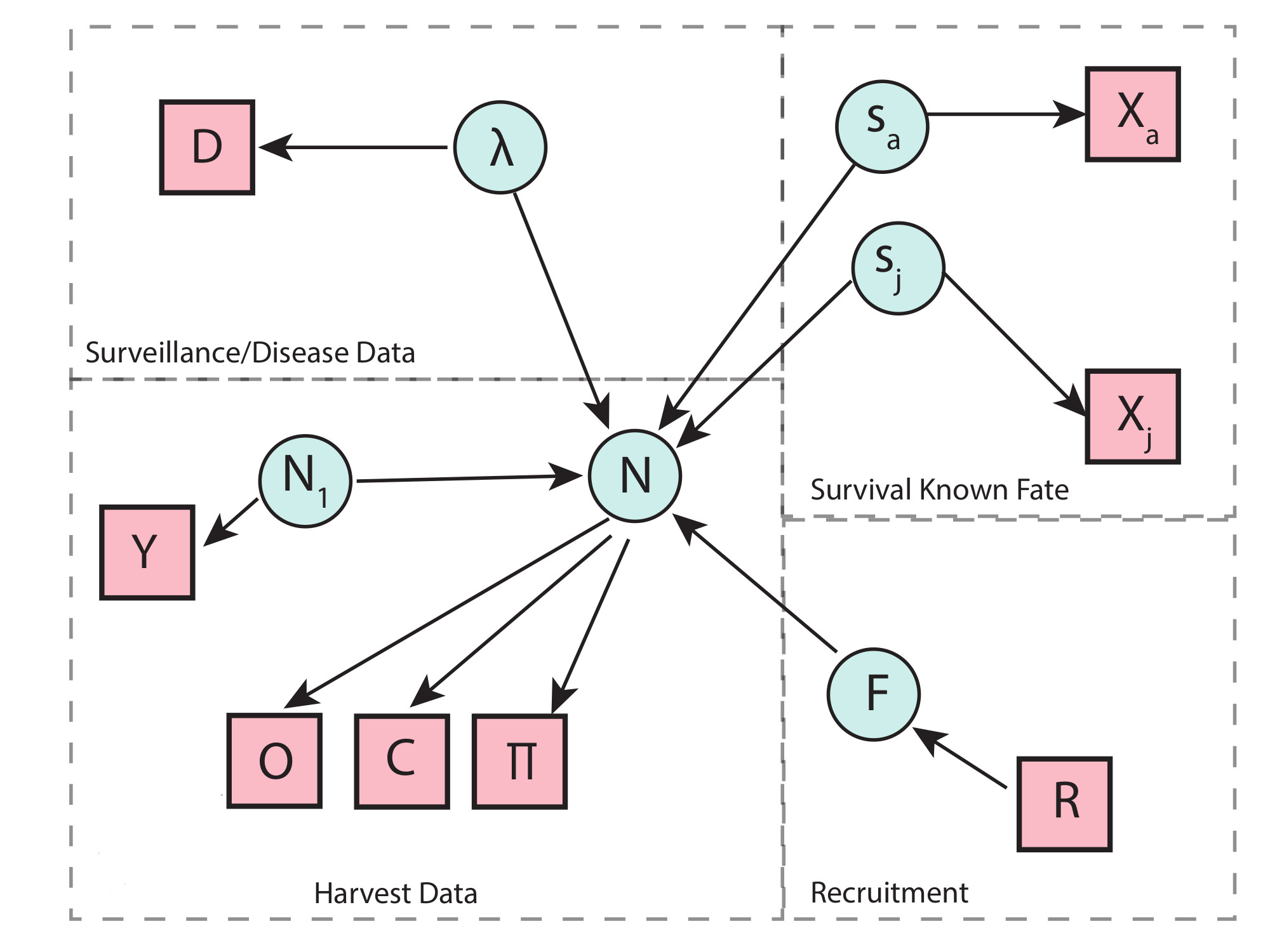
We are developing a spatial-temporal integrated population to asses the population impacts of chronic wasting disease on white-tailed deer in south central Wisconsin. To demonstrate population impacts, a pathogen must be shown to effect survival, recruitment, immigration or emigration rates. Integrated population models (IPM) combine multiple data types in a single unified analysis. These approaches combine survey and demographic data to understand population dynamics, incorporating life history elements by accounting for births, mortality and movements explicitly while propagating the uncertainty and variability associated with these processes in a combined framework (Besbeas et al, 2002, Brooks et al., 2004, Schaub et al, 2011, Zipkin and Saunders, 2018).

IPMs are generally constructed with three data sources consisting of (1) population abundance, (2) survival from mark-recapture, and (3) fecundity data, such as young of the year counts. For our study we have a related but different suite of data sources and demographic rate models, including hunter harvest data, camera trap data, and GPS collar data. Using the age-at-harvest data we can obtain deer density estimates for the IPM. Because of the high resolution of GPS location data, we have highly precise time of death information that we can model using continuous time-to-event known fate survival analysis.  We will use camera trap data and pregnancy rates to obtain measures of recruitment.

In our present study, we have the additional challenge of needing to model disease dynamics that are highly heterogeneous. CWD transmission has been shown to vary across age classes, sex, PRNP genotype, with spatial and temporal dependence. We will use surveillance data from hunter harvested deer that have been tested for chronic wasting disease since 2002.

Age-at-harvest population model

Cross-sectional harvest data are used to reconstruct population abundances of cohorts through time (Cross et al 2008, Fieberg et al 2009, Norton et al, 2017), based on latent process demographic parameters.

Process model

We will assume a Markovian state process, where the population density at time t + 1 depends on the population at time t, and a function (g) of parameters governing the ecological processes of survival (s) and reproduction (r). Many population models also account for immigration and emigration, although we make the simplifying assumption that the population is closed to these in/out processes. In general,

N_t+1 = N_t × g(s_t,r_t),

for year t = 1, …, T , where survival and recruitment vary by year. For the years we have collars deployed, 2017-2021, we will use posterior predictive distributions to obtain survival for non-hunting and hunting seasons annually. From 2005-2017, we’ll have a 12 year period where we don’t have mark-recapture data. We could average across the book-ending observations to obtain mean survival rates, assuming a constant survival for those in-between years. Similarly, provided the assumption of constant survival, we could use a moment-matched prior from the literature.

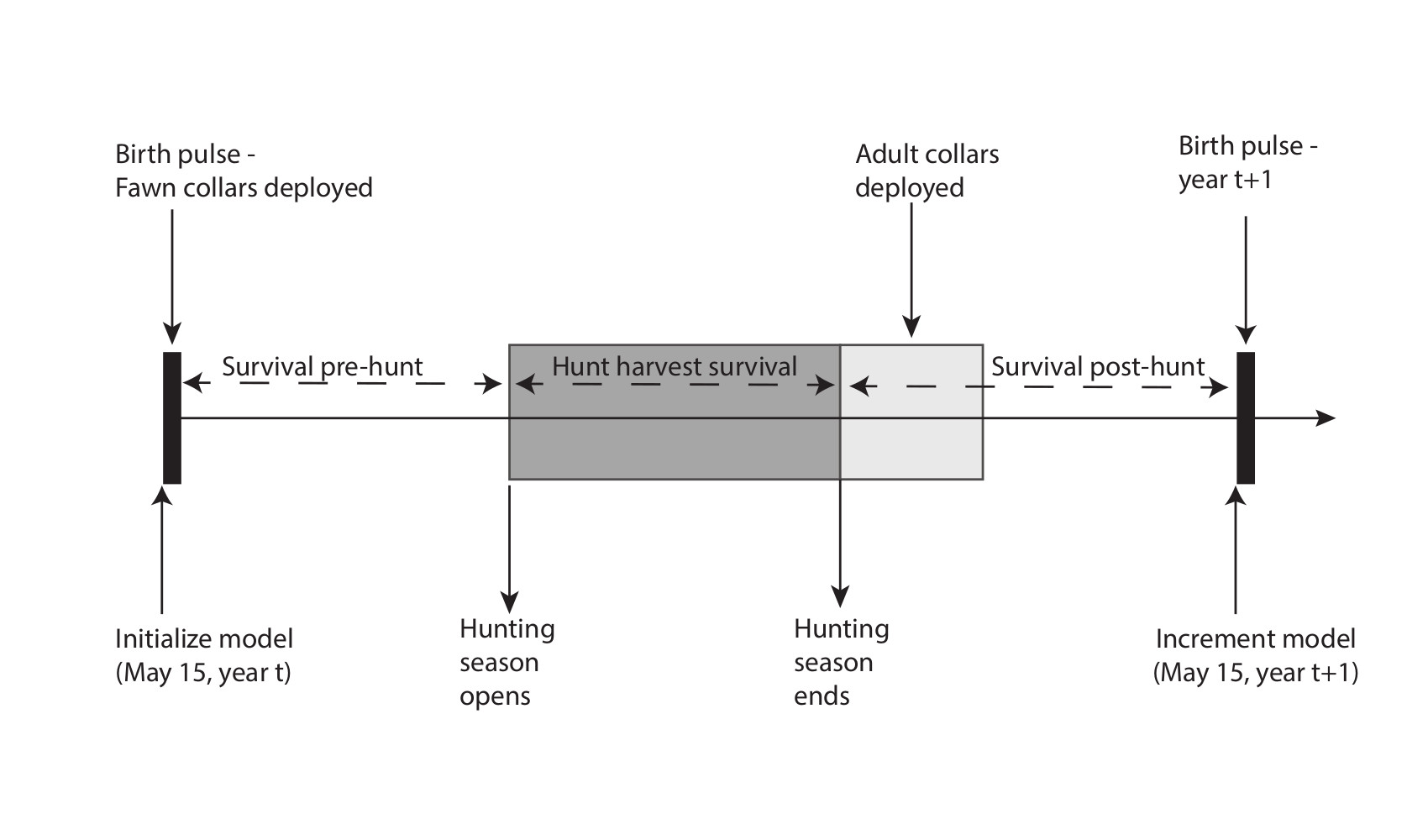
An annual timeline of events, similar to Fieberg et al. (2010) and Gast (2013), was created to help with formulating important phenomenon pertaining to the annual life cycle considering surveys/collaring, harvest, and the birth pulse.

The simplified population reconstruction using age at harvest data is given by

[insert matrix table here]

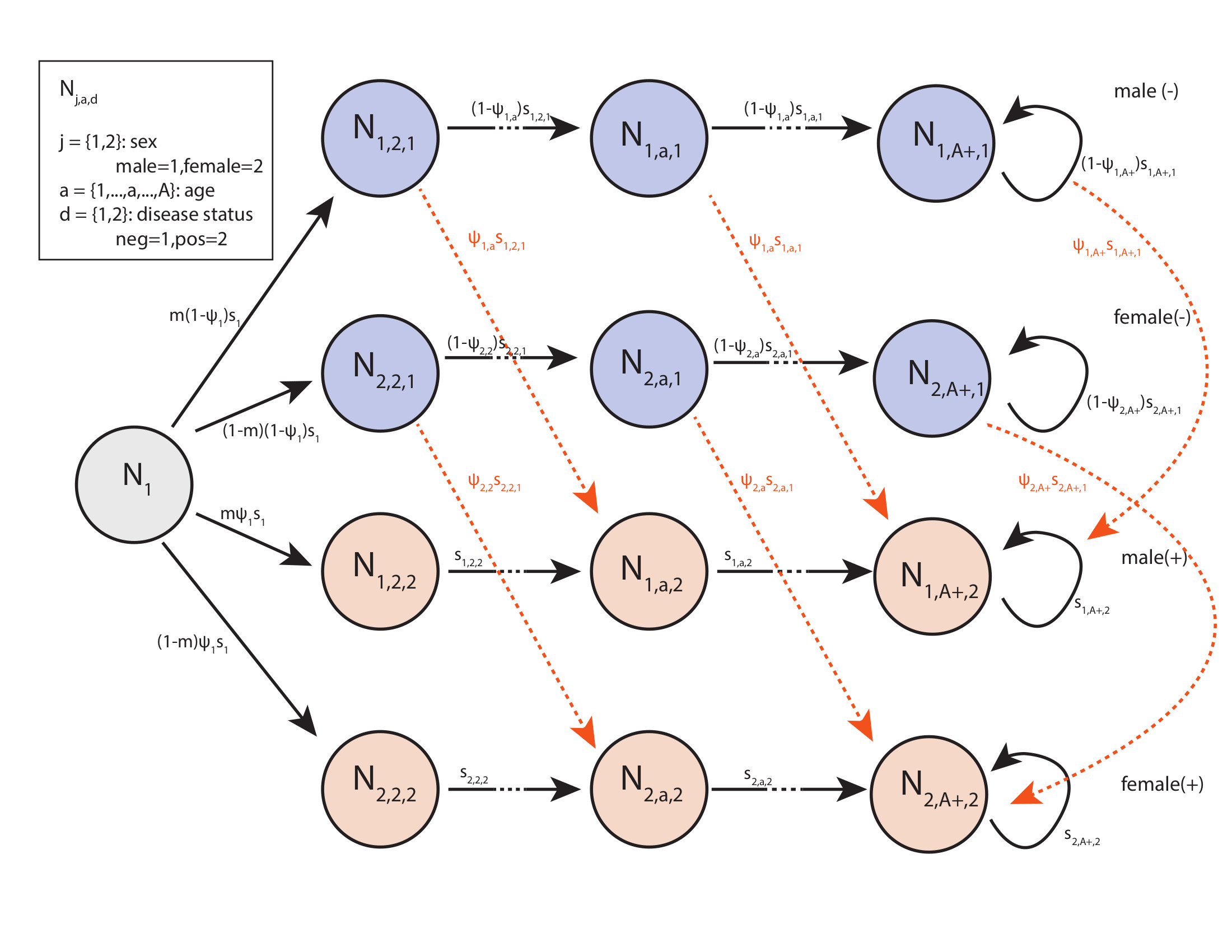
The following simplified life history diagram only incorporates disease status, age, and sex.

I’ve omitted study area to aid in viewing because this model grows in dimension quickly. Ultimately this process model is founded in a leslie matrix formulation, so all of the assumptions of that modeling framework apply here, including, for example Mathulsian population growth.

We will separate mortality during the hunting season, including bow and gun, from natural

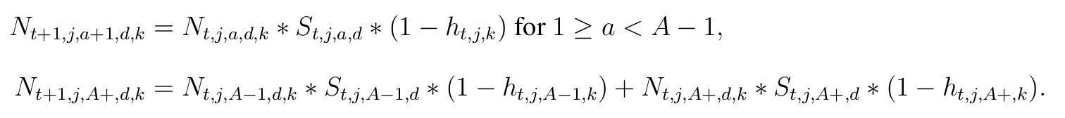
mortality outside of hunter harvest. Predicted “true” abundance for each state variable is given by a series of two equations. The second equation is necessary to account for the terminal age class, denoted (A+) representing the fact that individuals that are 12.5 years of age or older remain in that age class.

Population data sources/description

A challenge for this analysis is that the study areas and harvest records have different spatial ex-tents. In some years harvest is specified by section, that we can sum over to correspond with the total harvest from each study area precisely. In other years, harvest was reported at a county level, of which both study areas are a subset. We’ll have to use Arcgis to determine the total proportion of the study area that is a subset of each county, along with available habitat, in order to scale the data.

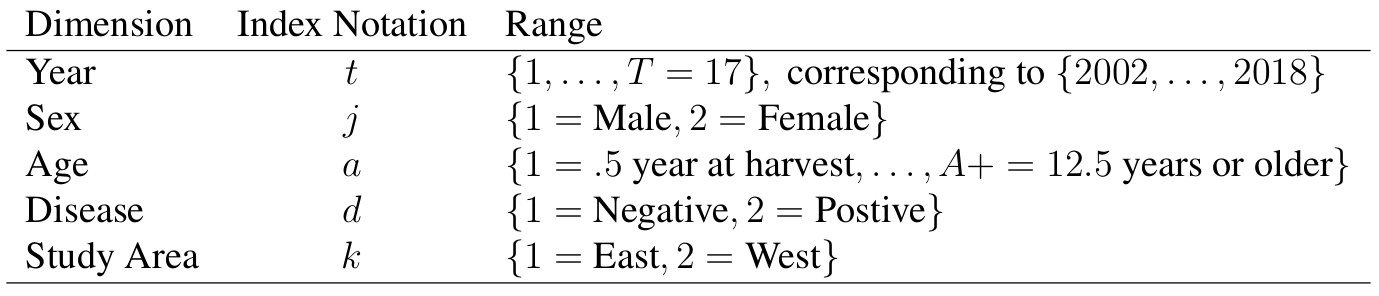
There are two sources of harvest data requiring separate likelihoods. These consist of observed antlered/antlerless total counts (O) and a subset of aged cohort data (C). First we consider the total observed harvest counts broken down into the two groups consisting of

• Antlered males (1.5 years of age or older)

• Antlerless group consisting of all individuals less than 1.5 years of age as well as adult and yearling females.

For the years 2002-2012, we have observed harvest of antlered/antlerless groups according to section. We can use the total from these sections that align with the study area boundaries (O). Thus these observed counts of anterled or antlerless harvested individuals are denoted O with dimensions (t) for years, j for group (antlered or antlerless), and study area (k), that is given by two independent normal distributions

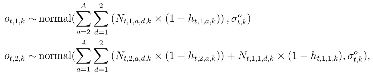
for t corresponding to years from {2002, …, 2012}, with observation variances (σ t,k) requiring priors. Note that in the likelihood, the sums occur over slightly different age cohorts for the two groups, reflecting young males being in the antlerless group with the second additive term. From 2012-present, the spatial extent of the harvest data differs, and is reported at the county level. We will have to scale the harvest by the proportion of the spatial area that is the study area proportion δ_k scaling the random variable counts, and is defensible because these terms are constant by study area. We can also include knowledge regarding hunter availability across the landscape here in our scaling. Thus, observed antlered individuals are given by

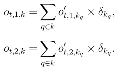
These derived classes can be modeled with a similar series of independent normal distribution likelihoods

for t corresponding to years from {2013, …, present}. Lastly, we’ll include a constant reporting rate term across all years that is consistent with other age-at-harvest models included Feiberg (2010) and Gast (2013).

Aged Harvest Data

The aged harvest data (C) consists of only a subsample of the total reported harvest, so we must assume that the subset is a representative sample of the ages of these cross-section data. These data are recorded on a county level, and there a few ways we could handle the mismatch spatial extent.

One approach would be to assume the stable stage distribution, i.e. the composition of age classes are the same between both study area. In which case, we would ignore the county separations and aggragate over all of them. Another approach would be to assume that the Iowa county plus Grant county compositions are representative of the west study area, and the Iowa county plus Dane county compositions are representative of the east study area. A third approach would be to multiply the corresponding county count by the proportion of the area that are in each study area, and then add the proportions of Grant and Iowa, or Iowa plus Dane for the corresponding west and east study areas.

The likelihood for C is given by

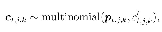
where  for l age classes, scaled, summed and rounded across the county level

data for each of the age classes.

Survival and Recruitment Analyses

Survival analysis is described to great detail under the survival section. Recruitment will be obtained using a combination of pregnancy rates from collared adult deer, fawn to doe ratios from WDNR staff, and fawn to doe ratios obtained from camera trap data.

Disease State Transition

We are in the process of developing spatial-temporal force of infection models from the surveillance data that we will describe in greater detail as we get further along in the model development process.

Literature Cited

Besbeas, Panagiotis, Stephen N. Freeman, Byron JT Morgan, and Edward A. Catchpole. “Integrating mark–recapture–recovery and census data to estimate animal abundance and demographic parameters.” Biometrics 58, no. 3 (2002):540-547.

Brooks, S. P., R. King, and B. J. T. Morgan. “A Bayesian approach to combining animal abundance and demographic data.” Animal Biodiversity and Conservation 27, no. 1 (2004): 515-529.

Fieberg, J. R., K. W. Shertzer, P. B. Conn, K. V. Noyce, and D. L. Garshelis. 2010. Integrated Population Modeling of Black Bears in Minnesota: Implications for Monitoring and Management. PLOS ONE 5:e12114.

Gast, C. M., J. R. Skalski, J. L. Isabelle, and M. V. Clawson. 2013. Random Effects Models and Multistage Estimation Procedures for Statistical Population Reconstruction of Small Game Populations. PLOS ONE 8:e65244.

Schaub, Michael, and Fitsum Abadi. “Integrated population models: a novel analysis framework for deeper insights into population dynamics.” Journal of Ornithology 152, no. 1 (2011): 227-237.

Zipkin, Elise F., and Sarah P. Saunders. “Synthesizing multiple data types for biological conservation using integrated population models.” Biological Conservation 217 (2018): 240-250.