Introduction and Methods

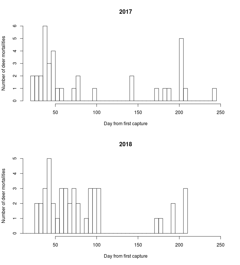
We estimated juvenile white-tailed deer survival using data collected from the first two years of the WIDNR southwestern deer study. During that time, fawns were captured and radio-collared in May and June of 2017 and 2018. Individual survival status was checked daily. Fawn survival was modeled in the same time-to-event Bayesian framework used to model adult survival (Walsh et al., 2017). We used a daily time step for the fawns, because mortality following birth is highly variable, and occurs on a shorter time span than for adults. We used a regularized version of the hazard model, with an ICAR (intrinsic conditional auto-regressive) effect for age. This differs from last year’s analysis, where we applied an ICAR effect along the time line starting mid-May. We imputed age at capture of the fawns because the exact age at capture is not known precisely. Fawns are typically too fast to capture more than 2 days (approximately) after birth, so we subtracted a randomly drawn value from a discrete uniform [0,2] distribution to account for the unknown age at capture in the hazard. We used a mixed model random effect along the time axis to account for daily variability across the two years that could contribute to changes in survival over time.

All models were fit using Bayesian methods and implemented in nimble (NIMBLE Development Team, 2019), with standard diagnostics indicating no evidence for non-convergence. A truncated normal prior was used for the intercept (β₀’), along with an additional mixing parameter (α) to help with convergence, such that

The lower (2.5%) and upper (97.5%) quantiles of the inverse of the complementary log-log (cloglog) transformation of the prior distribution for β 0 were 0 to .99, providing a prior distribution across the full range of likely survival values. The ICAR prior for the daily age effect was

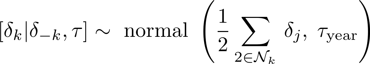
for k = 1,…,K days old, where δ_−k is all the elements of δ except the kth element, the neighborhood N_k is the set of 2 days that neighbor k, and was parameterized in terms of precision (τ_year). The linear model for the log hazard of the model with the gun harvest fixed effect was given by

for the jth individual during the kth age, where ε_i represents the random effect for k‘ day within the ith year given by

Model variations

We fit multiple versions of the random time effects model, and evaluated a shared precision structure rather than separate precision parameters for the annual time effects. We compared these results using WAIC values (Watanabe Akaike Information Criterion) for model selection (Hooten & Hobbs, 2015) and ultimately decided to use separate precision parameters for each year within the random time effect.

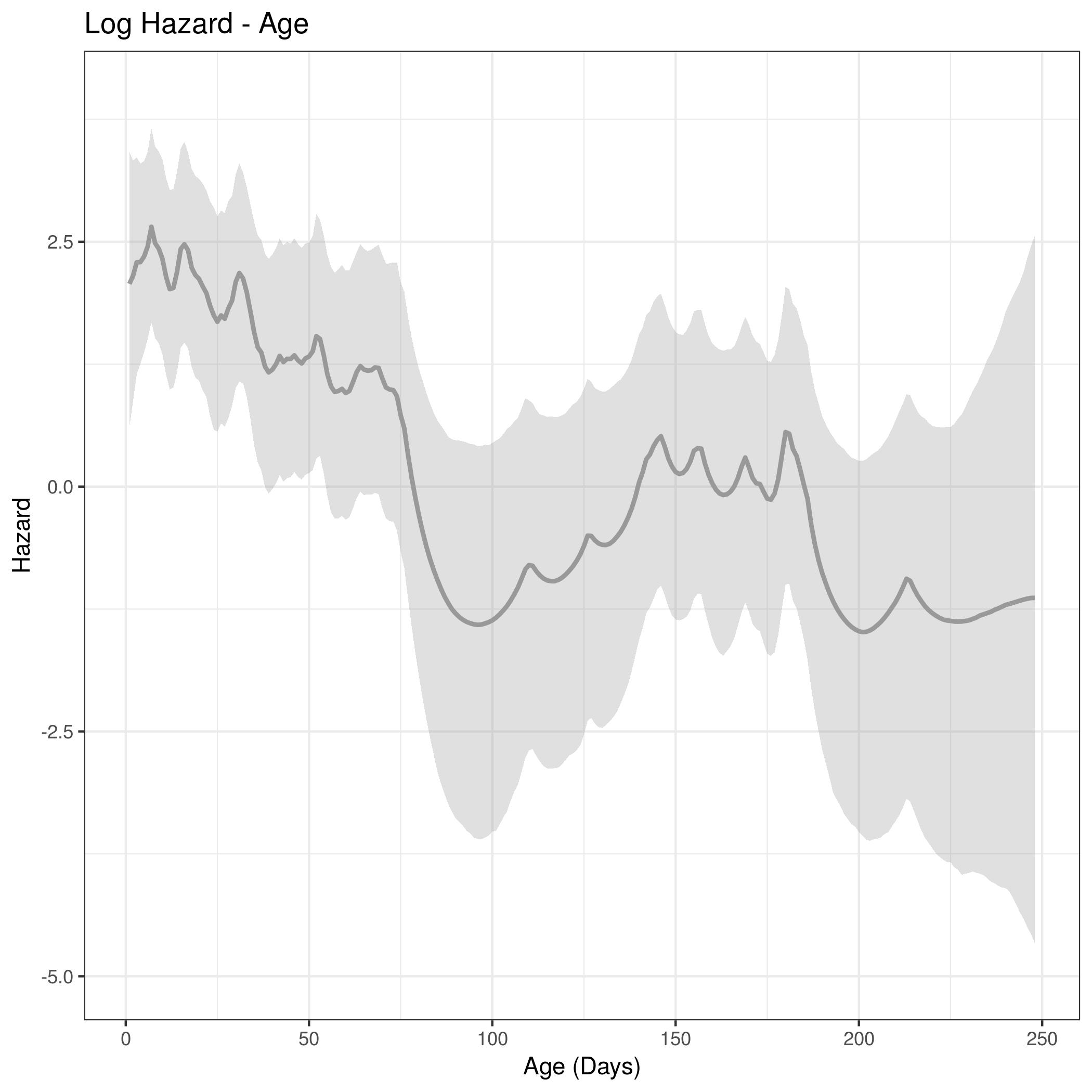
We observed that the posterior distributions of the log hazard along the age axis showed an increase in mortality during the hunting season. This increase in mortality partially reflects time of year (hunting season), rather than actual increases in mortality with age. Thus, we fit two model variations to incorporate fixed effects for gun harvest, and bow harvest, along the time axis to mitigate this increase in the log hazard.

We also tried an alternative prior formulation for the intercept, by providing a prior in the cloglog space of the intercept (i.e. a baseline survival probability using a flat uniform(0,1) distribution, then transforming this value to the log hazard scale. We found that convergence diagnostics were improved using the truncated normal formulation rather than the cloglog formulation. Parameter estimates were consistent between both models, supporting the conclusion that the truncation is not affecting model estimates.

Results: Juvenile Survival

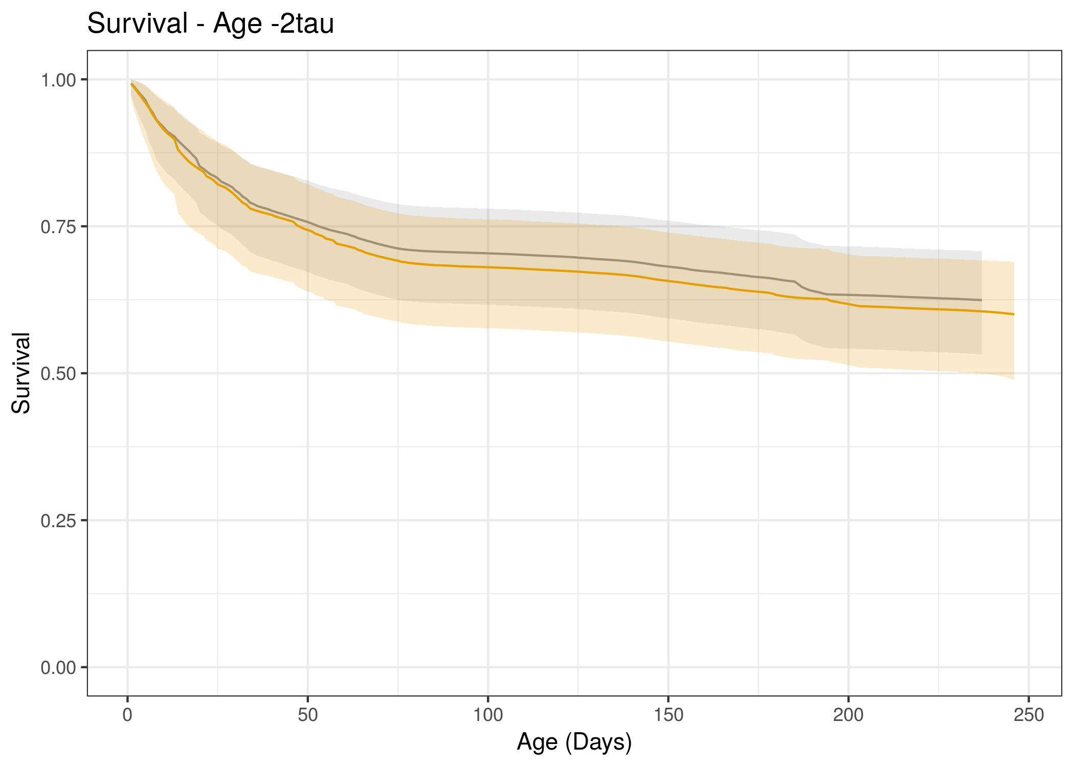
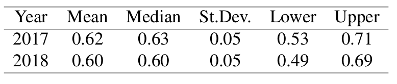
Juvenile survival estimates were estimated up to the maximum age observed at the end of the calendar year, which was 236 days old for 2017 and 248 days old for 2018. The maximum age varied because the first day of fawn capture differed across years, while fawn monitoring continued through the end of the following December and was equivalent for both years.

Hazard Results

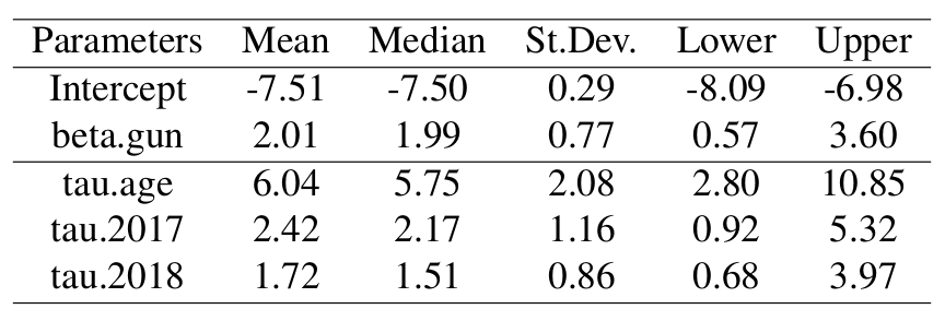
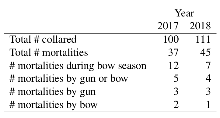
Posterior distributions of the coefficients in the hazard rate models were obtained for the intercept and gun harvest. The coefficient for gun harvest in the hazard was positive, indicating an increase in mortality resulting from harvest, as we would expect. The fixed effect for gun harvest was pooled across years because there were only 3 mortalities each year resulting from gun harvested fawns. Posterior distributions of the precision parameters for the daily age effect from the ICAR model, and for the random annual time effects were also obtained and summarized in the following table.

Conclusion

Fawn survival was nearly equivalent for both years, with substantial overlap of credible interval bounds. We cannot be sure if this pattern will continue because so far there are only two years of data. There are numerous factors that may be driving the high rate of fawn survival, although we have not addressed them with this preliminary analysis. As we collect more data we will implement a cause-specific mortality analysis.

Literature Cited

Hooten, M.B. & Hobbs, N.T. (2015) A guide to Bayesian model selection for ecologists. Ecological Monographs 85, 3–28.

NIMBLE Development Team (2019) NIMBLE: MCMC, Particle Filtering, and Programmable Hierarchical Modeling.

Walsh, D.P., Norton, A.S., Storm, D.J., Van Deelen, T.R. & Heisey, D.M. (2017) Using expert knowledge to incorporate uncertainty in cause-of-death assignments for modeling of cause-specific mortality. Ecology and Evolution 8, 509–520.